|
<< Click to Display Table of Contents >> Historical simulation |
  
|
|
<< Click to Display Table of Contents >> Historical simulation |
|
This section describes how to perform a historical simulation on a (historical) databank. In order to follow the examples, you must first download the model and databank (click demo.zip, and copy the two files gekko.frm and gekko.gbk into your Gekko working folder). The example uses annual data, but other frequencies would run very similarly.
(See the bottom of this page for the full code).
Start up Gekko in the working folder.
Then type this in the statement prompt (at the bottom):
restart; mode sim; |
If you copy-paste these statements to Gekko, you may either execute them individually one by one by pressing [Enter], or first mark them as a block and then press [Enter] to execute them at once.
The statements clear up the workspace, and set the global time period (for which we will later simulate the model). At the bottom of the Gekko window, you can see that this time period has been set ("Annual 2004 2016"). You may try to load the model, read the data variables, and print them out:
model gekko; |

The first statements load gekko.frm and read the gekko.gbk databank file. Note the use of the < and > brackets denoting local options. In all relevant statements, you can state a time period inside such brackets, and the given time period will only be used in that statement. The PRT statement prints both levels and annual growth for the variables. (Note the codes (E) for endogenous, and (X) for exogenous).
The data is articifial, and contains no growth. So the model can be envisioned as either depicting a stationary-state model (with dynamics), or depicting growth-corrected variables. Avoiding growth in the data is just to keep the model simple.
Lists may be used to avoid repetitive typing:
#vars = y, c, x, g; |
Try printing out the current lists:
list ?; |
This shows the newly created list #vars. There are also some model lists. For instance, the list #all contains all model variables, #endo contains all endogenous variables (i.e., variables at the left-side of an equation), and #exo contains all exogenous variables (to see the contents of the #exo list, use PRT #exo;). Now you may print the variables using the list (instead of prt y, c, x, g;):
prt {#vars}; |
Note that prt #vars; would print out the list itself (that is, four strings). Instead of lists, wild-cards can be used, for instance:
prt {'*'}; |
This will print out all timeseries in the Work databank. The alternative prt ['*']; would print out the variables as strings (names). Note that there are some model-created variables (dummies, add-factors, with missing values (M)) — these will be described later on. Wildcards follow the standard: * for any match, and ? for single character match.
We will now try to simulate the model. It should be noted, that any READ statement works like this: First the Work databank is cleared, and the databank file is read. Next the Ref databank is cleared too, and all variables in Work are copied into Ref. Hence, after any READ statement, the two databanks Work and Ref are always identical. (You may use READ<merge> to merge data, or READ<ref> to load data into the Base databank separately). To verify this, try to print a multiplier difference:
mulprt {#vars}; |
As you can see, there is no difference. This will change after we simulate the model:
sim; |
![]()
The SIM and MULPRT statements are executed over the period 2004-2016 since this is previously set as the global time period. As expected, for g there is no difference (it is exogenous), whereas there are differences for the other variables (the simulation is dynamic: a static simulation using historical values for lagged endogenous variables can be done with SIM<static>). To see the data more clearly, you may try:
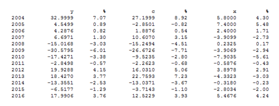
prt @y, y; |
The symbol @ indicates that the value is taken from the Ref databank. Alternatively, try:
mulprt <v> y; |
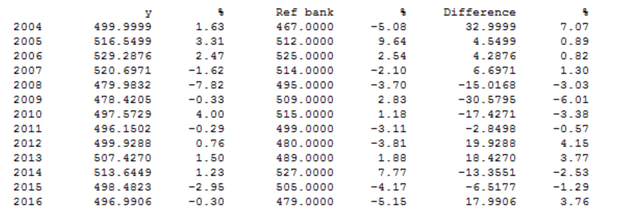
which prints out both Work and Ref values, and multiplier differences (v means 'verbose'). Instead of printing, you may create a graph with PLOT:
plot @y, y; |

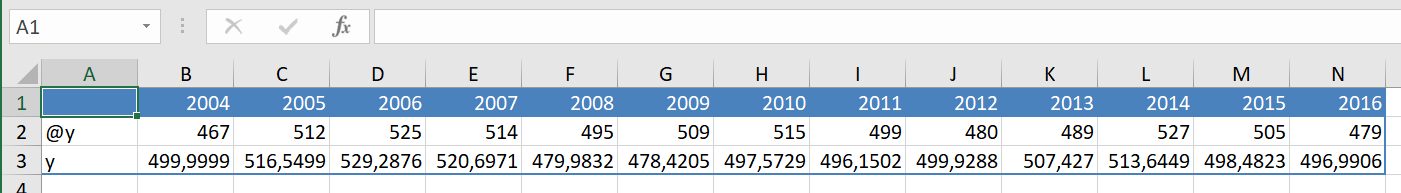
In general, you may substitute PLOT for PRT, since the syntax is identical. In the window, you may for instance try to click the p (growth rate) radio button, and you may use [Esc] to close a graph window quickly. Instead of PLOT, you may also try SHEET, which shows the data as an Excel table (if Excel is available on the computer, else use CLIP).
In general, for statements like PRT, PLOT, SHEET and CLIP, you may use so-called "operators". For instance, p means annual growth rate, m means absolute multiplier differences, and q means relative multiplier differences. So this statement:
prt <p> {#vars}; |
will print percentage annual growth rates for the variables, and
plot <p> {#vars}; |
plots them. You may also use a r to indicate Ref databank, for instance:
prt <rp> {#vars}; |
This prints percentage change and levels for the Ref databank.
If you wish to store the result, you may write it to a databank (.gbk file):
write simple; |
This will store the file simple.gbk in the Gekko working folder. Later on, you could read it with read simple;.
In sim-mode, any new variable not present in the model should be created first (unless the variable name starts with xx, in which case the variable will be auto-created as a convenience):
create g2; |
The statement makes g2 and g identical, for the given period. Another expample could be this:
pch(g2) <2003 2016> = pch(c) - pch(y) + 2; |
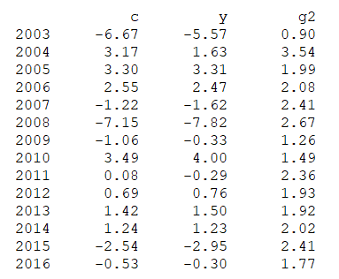
The first statement (a SERIES statement) is set to start in 2003 — otherwise the result will be missing values, since the pch() function uses lagged values. Note also in the PRT statement the p inside the option brackets for indicating annual percentage growth rate. As it is seen, the annual growth rate of the new g2 variable is set to the growth rate of c minus the growth rate of y plus 2 (percentage points).
The PRT/PLOT/SHEET/CLIP statements accept any expression, so the historical consumption rate may be printed like this:
prt <r> c/y; |
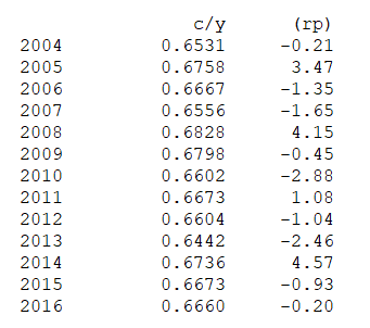
where the operator r indicates Ref (reference/historical) values: prt @c/@y; or prt ref:c/ref:y; could also be used. Another way of printing variables is the DISP statement. This statement does not accept mathematical expressions, but prints the equation (if it is an endogenous variable), variable explanations (labels), etc. Try:
disp y; |
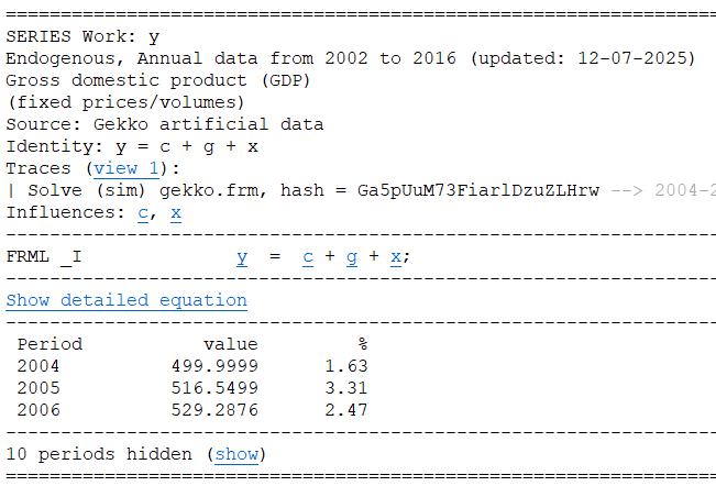
You can see the GDP equation, and the label associated with the y variable (this label is taken from the .frm file, after the VARLIST$ tag). You may follow the links by clicking the underlined variables, like in a web browser. Use the arrow buttons at the top-left of the Gekko window to browse backwards and forwards.
Another way of showing information regarding endogenous variables is using the DECOMP statement. Type:
decomp y; |
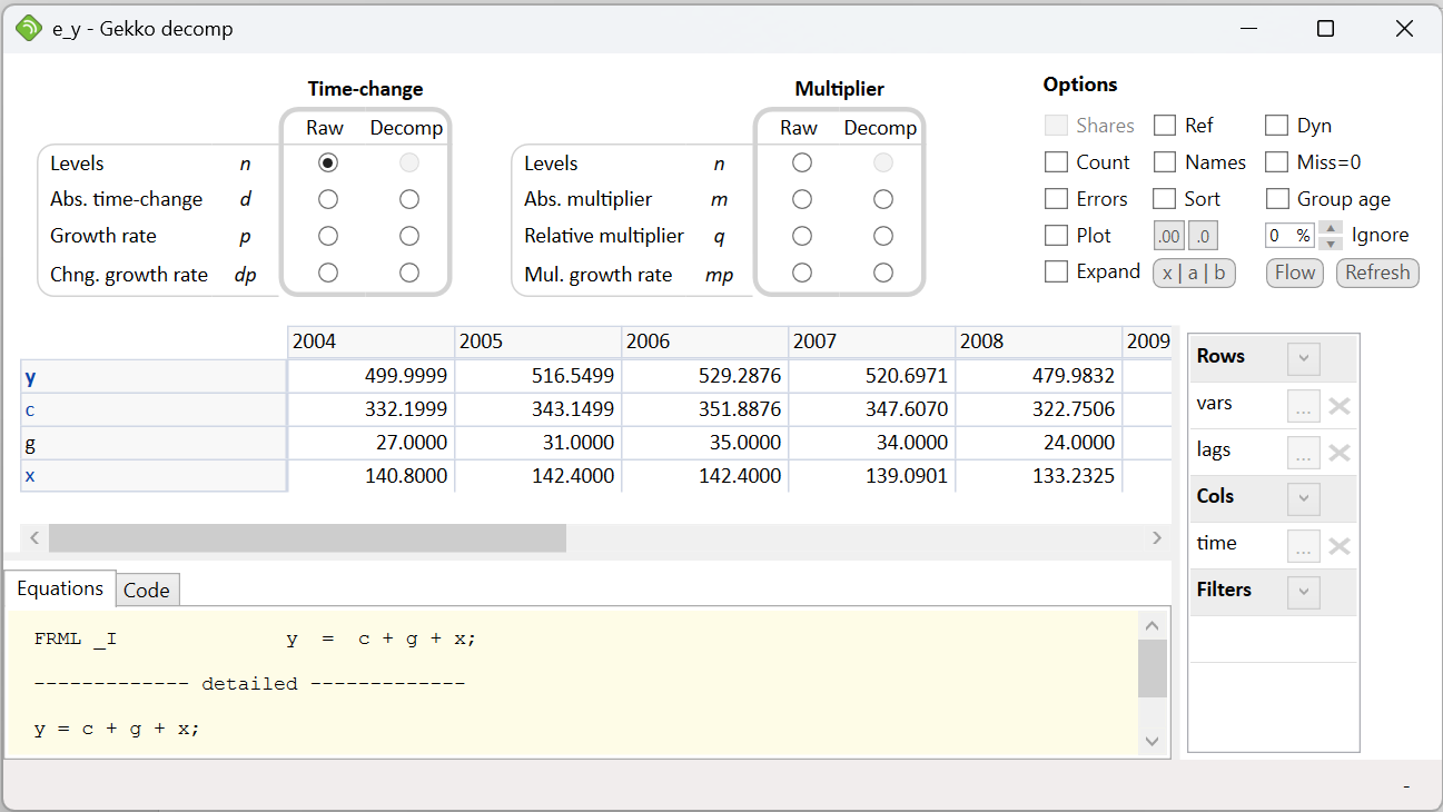
This opens up the decomposition window, showing the variable values, and the values of determining variables (precedents). Cells may be marked and copy-pasted to Excel or other spreadsheets. The first line of the table is the dependent variable (left-hand side of equation), whereas the following lines are the explanatory variables (right-hand side of equation).
If you click Growth rate (p) in the Raw column under Time-change, the values are shown in annual percentage growth rates. For instance, in 2004, the simulated value of y grows with 1.63%, whereas private consumption c grows with 3.17%. The percentages regarding c, g and x obviously do not sum up to the 1.63%, which can be verified by marking the three cells, and looking at the status bar at the bottom of the window (reporting 8.27% in total). However, if you click the same button in the Decomp column, the percentages regarding c, g and x sum up, because the contributions in the equation are "decomposed". So, in 2004, the simulated value of GDP growth (1.63%) is composed of +2.07% of c-contribution, +0.41% of g-contribution, and -0.85% of x-contribution. That is, it is the private consumption (c) that is driving the growth in y in 2004, whereas net exports (x) pulls in the opposite direction (you may click Show as shares to easier spot which variables contribute the most to the changes in y).
If you alternatively click Abs. multiplier (m) in the Raw column under Multiplier, the absolute multiplier is shown (i.e., the absolute difference between the historical databank and the simulated values, corresponding to MULPRT or PRT<m>). For instance, in 2004, the simulated value of y is 33 units larger than the databank value. The multiplier part of the decomposition window is most often used in multiplier analysis, i.e. analyzing two simulated scenarios.
Click the Flow button to open up the flowgraph viewer:
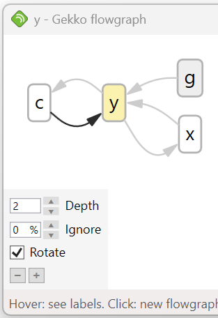
Flowgraphs can be very convenient for larger models. Note that DECOMP and flowgraphs also works for GAMS equations/models.
The full code
restart; |