<< Click to Display Table of Contents >> Navigation:  Gekko User Guide > Modeling User Guide > 4. Multiplier analysis (shocks)

This section describes how to perform forecast scenarios, based on a historical databank. In order to follow the examples, you must first download the model and databank (click demo.zip and copy the two files gekko.frm and gekko.gbk into your Gekko working folder).

 

(See the bottom of this page for the full code).

 

Next start up Gekko in the working folder, and type:

 

 

This clears up the workspace, and sets the global time period (for which we will later simulate the model).

 

 

The first statements load gekko.frm and reads the gekko.gbk databank file. The databank file only runs to 2016, since 2016 is the last historical data point. Like in the previous section, create a list containing the variables:

 

 

As you can see, the variables contain all missings (M) for the period 2017-2040. We will now try to simulate the model (for 2017-2040):

 

 

Gekko will complain about missing data (click the link in There were missing values in 1 variables, and afterwards click the Main tab again to get back (or use Ctrl+M)). So as stated in the Output tab, the problem is that the value of g for the period 2017 is needed in order to simulate for 2017. Try setting g constant (for the global period 2017-2040) by means of the SERIES statement:

 

 

The %= operator in the first statement sets annual percentage growth, and after this, the model can simulate. The model is really quite simple: as seen in the x-equation, x will always change unless y = 500. So this value for y is an equilibrium value (attractor), for instance corresponding to zero (or natural/structural) unemployment level.

 

The equilibrium level of the consumption equation is given by c = 0.6/(1-0.1)*y, corresponding to 0.6/0.9*500 = 333.33. Net exports are given residually, from the GDP identity. Hence in equilibrium, x = y – c – g = 500 – 333.33 – 31 = 135.67. The interpretation is that in the long run there is perfect crowding-out regarding public consumption g, since 1 extra unit of g will entail 1 less unit of x. As it can be seen from the above PRT statement, the actual values converge slowly to these long-run values.

 

If the best prognosis regarding future government consumption is that it is unchanged at at 31 units, this simulation can be considered a reference scenario. In order to perform a multiplier analysis on top of this reference scenario, we need to put the scenario into the Ref databank (in order to be able to compare it to the alternative scenario later on). Try printing all values for the variable y (operator v means 'verbose'):

 

 

As it is seen, there are missing values in the Ref databank. The CLONE statement copies data from Work to Ref, so try this:

 

 

As it is seen, Work and Base databank values are now identical, and we are ready to perform an alternative simulation.

 

The experiment is the following:

 

 

The operator +=  adds to the value in the Work databank, so in each year, g is augmented by an absolute amount of 100 relative to the baseline values. The alternative scenario is simulated:

 

 

Instead of printing, we will use the graph facilities. Try the following statement:

 

 

We start out changing the global time period to 2016-40, so that the last historical year is included in the following prints and plots. The plot shows the simulated values (levels), not the multiplier (differences). For instance, you can see that g changes from 31 in 2009 to 131 in 2016, as expected.

 

Now, in the graph window, try to select Abs. multiplier (m), in order to see the multiplier.

 

 

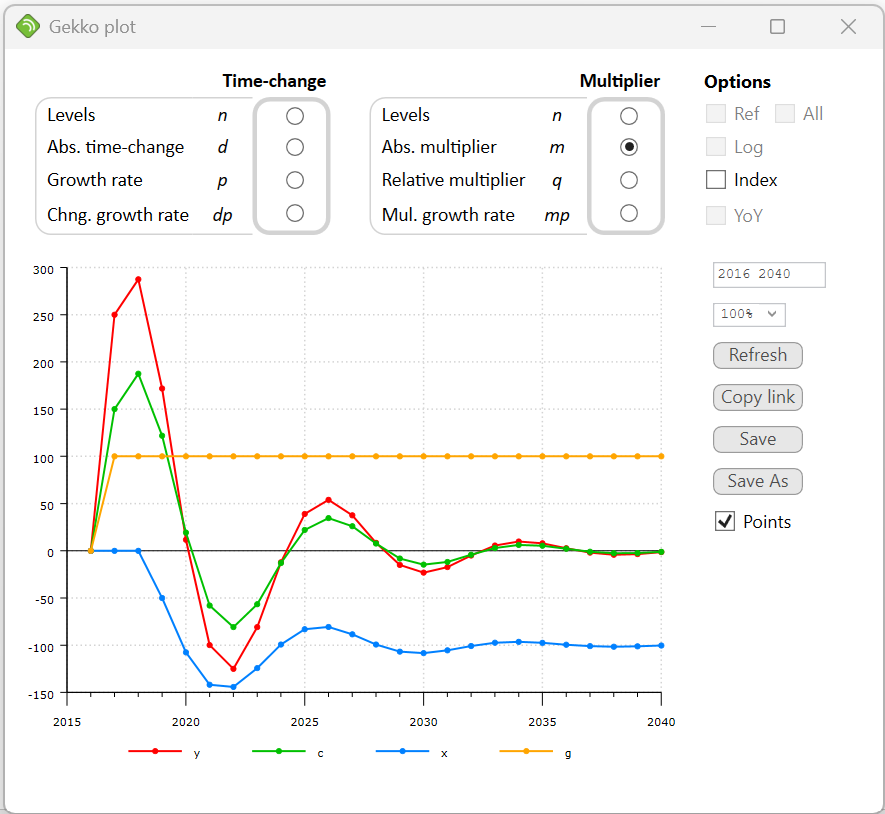
Government spending (g) changes permanently with 100 units, and in the first year this creates a Keynesian extra effect on production (y) which increases with 250 units. The effect on private consumption (c) is 150 units.

 

The effect is augmented a little bit more the following year, because of the lagged endogenous term in the c-equation. From 2019 and on, however, the net exports begin to decline (the effect propagates via the term y(–2) in the x-equation). The underlying interpretation could be that — with some delay — the rising production lowers the unemployment rate and thus augments the wage levels. This in terms puts an upwards pressure on the domestic price level, lowering net exports. This negative effect on x pulls y back downwards, and as it is seen, y oscillates slowly back to its former level (i.e. the multiplier is 0 in the long run, corresponding to full crowding-out).

 

So in the long run, y and c are unchanged, whereas g has been augmented by 100 and x reduced by 100. So, as mentioned above, in the long run the increased government consumption is exactly crowded out by an equivalent reduction in net exports.

 

If, instead of Abs. multiplier you select Relative multiplier (q) in the graph window, you can see the percentage multiplier differences. The effect on g is quite large in percentages, whereas y and c follow each other quite closely in percentages. It is worth noting that you may call PLOT with an operator to indicate how the data should be presented, for instance:

 

 

The m operator code indicates absolute multiplier, i.e., the absolute difference between the two databanks. The same code can be used for PRT, for example:

 

 

Also, instead of PRT or PLOT, you may use SHEET, provided that Excel is installed on your computer (otherwise use CLIP):

 

 

This creates an Excel sheet with the data. In Excel, a graph is easy to create from this table (for instance, in Excel 2019, you can click on any cell inside the table, choose "Insert", and then choose a graph). As a side note, you may create the Excel file automatically without opening up Excel:

 

 

This will silently create the file simple.xlsx and put it into your working folder. Note the labels on each variable. You may also use expressions as you wish, for example:

 

 

This show absolute multiplier changes in these three rates.

 

Other convenient operators in addition to m are p for annual percentage growth, and q for multiplier percentage change.

 

You may also use the DECOMP facility to analyze equations and contributions. For instance:

 

 

This starts the decomp window: try clicking Abs. multiplier (m) in the Raw column of the Multiplier section. This will show multiplier values related to the y-equation.

 

 

 

The full code