The R_RUN statement is used as an interface to R. The interface allows easy transfer of matrices from Gekko to R, execution of a R program, and easy returning of matrices from R to Gekko. Instead of matrices, you may alternatively use Apache Arrow files to communicate with R, cf. the example at the end of this page.

Compatibility note regarding syntax:

Starting with Gekko 3.1.8, the R interface syntax is simplified, and the former statements R_FILE, R_EXPORT are no longer needed. If you are using the deprecated syntax, you may easily upgrade to the new syntax. For instance, you may translate R_FILE ols.r; R_EXPORT <target = 'data1'> #x, #y; r_run; into simply r_run <target = 'data1'> #x, #y file = ols.r;, merging the three statements. The old syntax will work for a while, but please consider converting to the new syntax.

When executing R_RUN, you need R on your system, and Gekko will attempt to auto-detect the location of R. If this fails, you may indicate the location via option r exe folder = ... ; (Gekko will automatically add R.exe or \R.exe, unless the path ends with .exe, .bat or .cmd). If you just need to export matrices for use in R (without returning to Gekko), try the EXPORT<r> statement. Regarding an equivalent interface to Python, see PYTHON_RUN.

Syntax

r_run <MUTE TARGET=...> matrix1, matrix2, ... FILE = filename ;

r_run <MUTE TARGET=...> filename ;

MUTE	(Optional). With this option set, R is run silently in Gekko. Alternatively, R output is shown in the Gekko main window. Do not used <mute> when debugging your R program, since it shows potential R error messages.
TARGET =	(Optional string). If for instance <target = 'data1' >, the matrices are inserted at the exact location in the R file, where there is a line starting with gekkoimport data1. If the option is not given, the matrices are inserted at the top of the R file (this is often sufficient, the target logic is intended for larger R programs)
FILE =	Filenames may contain an absolute path like c:\projects\gekko\bank.gbk, or a relative path \gekko\bank.gbk. Filenames containing blanks and special characters should be put inside quotes. Regarding reading of files, files in libraries can be referred to with colon (for instance lib1:bank.gbk), and "zip paths" are allowed too (for instance c:\projects\data.zip\bank.gbk). See more on filenames here.

Example syntax:

r_run <target = 'data1'> #x, #y file = ols.r;

Example

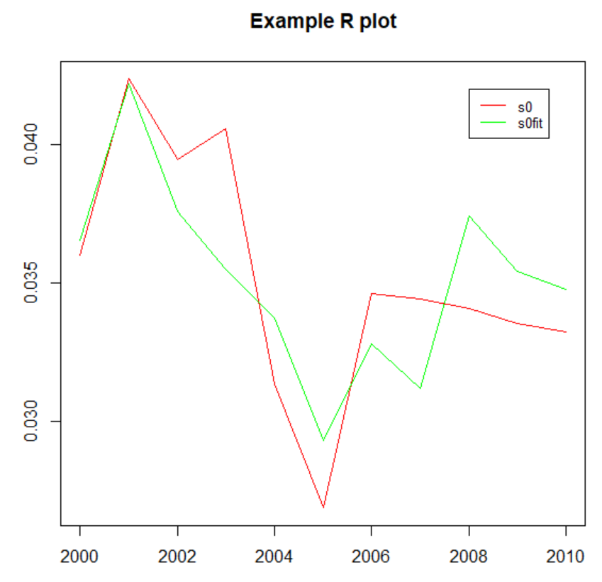
The example below estimates (in R) a linear least squares model with five parameters. You may consult the OLS section to see the same parameters calculated via the OLS solver, or the MATRIX section to see the same parameters calculated via linear algebra. See also the Python interface.

First, put the following R file ols.r into your working folder:

gekkoimport data1 # Gekko data (matrices x and y) is inserted here
fit <- lm(y ~ x)     # ols estimation
summary(fit)     # prints output
beta <- fit$coefficients   # estimated parameters
yfit <- fit$fitted.values # predicted values for y
gekkoexport(beta)   # writes beta vector back to Gekko
gekkoexport(yfit)   # writes fitted values back to Gekko

# ---------- example of plotting via R ----------
# somewhat convoluted because Rscript.exe is used as the R engine, therefore showing a plot
# window is a bit more difficult than using for instance RStudio.
library(tcltk)
windows()
t = seq(2000, 2010)
plot(t, y, type="l", col="red", ann=FALSE)
lines(t, yfit, col="green")
title(main="Example R plot")
legend(2008, 0.042, legend=c("s0", "s0fit"), col=c("red", "green"), lty=1:1, cex=0.8)
capture <- tk_messageBox(message = "")

Next, you can run the following program in Gekko:

reset; cls;
lna1 <1998 2010> = data('166.223000 173.221000 179.571000 187.343000 194.888000 202.959000
  209.426000 215.134000 222.716000 230.520000 238.518000 246.654000 254.991000') ;
pcp <1998 2010> = data('0.9502030 0.9699920 1.0000000 1.0235000 1.0401100 1.0605400
  1.0754700 1.0977800 1.1121200 1.1314800 1.1513000 1.1717600 1.1871600') ;
bul1 <1998 2010> = data('0.0684791 0.0591698 0.0560344 0.0535439 0.0535003 0.0631703
  0.0649875 0.0578112 0.0473207 0.0404508 0.0467488 0.0472923 0.0475191') ;
%t1 = 2000;
%t2 = 2010;
time %t1 %t2;
s0 = dlog(lna1);
s1 = dlog(pcp);
s2 = dlog(pcp.1);
s3 = bul1;
s4 = bul1.1;
#x = pack(%t1, %t2, s1, s2, s3, s4); //matrix
#y = pack(%t1, %t2, s0); //matrix
r_run <target = 'data1'>  #x, #y file = ols.r; //returns matrices #beta and #yfit from R
prt #beta;
s0fit = #yfit[.., 1].unpack(%t1, %t2);
plot s0, s0fit;

The program prints R output on the screen, and plots actual and predicted values. Plotting is done using both R's plot function, and Gekko's own PLOT (the R plot is shown below).

clip0039

The #beta vector looks like this:

#beta
   1
   1 0.0298
   2 0.1445
   3 0.6139
   4 0.1867
   5 -0.3509

Some of the output from R shown in Gekko is the following (cf. the same example in the OLS section):

Coefficients:
Estimate Std. Error t value Pr(>|t|)
(Intercept) 0.029804 0.008942 3.333 0.0157 *
x1 0.144517 0.227011 0.637 0.5479
x2 0.613875 0.236473 2.596 0.0409 *
x3 0.186740 0.202534 0.922 0.3921
x4 -0.350908 0.203182 -1.727 0.1349
---
Signif. codes: 0 '***' 0.001 '**' 0.01 '*' 0.05 '.' 0.1 ' ' 1

Residual standard error: 0.003462 on 6 degrees of freedom
Multiple R-squared: 0.625, Adjusted R-squared: 0.3751
F-statistic: 2.5 on 4 and 6 DF, p-value: 0.1516

Note that in this example, the <target= 'data1'> option and the corresponding gekkoimport data1 in the ols.r file are not really necessary, since the data could just be put at the top of the R file anyway. The code that is injected into the R file before it is executed looks like the following:

x = c(0.0304674549413991, 0.0232281261192072, 0.0160983506716728, .... )
dim(x) = c(11, 4)
y = c(0.0360024370055795, 0.0423704884205201, 0.0394838732643257, .... )
dim(y) = c(11, 1)

And the file that R produces for Gekko to consume looks like the following (this is actually what the gekkoexport() function in R does):

R2Gekko version 1.0
-------------------
name = beta
rows = 5
cols = 1
0.02980389
0.1445173
0.6138751
0.1867401
-0.3509083
-------------------

...

This text-based way of interchanging data back and forth works fine, as long as the datasets are not too voluminous (otherwise see the following section). The interface is more stable than COM-based automation, and interchange of values, text, etc. could also be provided if needed.

Apache Arrow files

As an alternative to matrix-based communication with R, Gekko also supports the so-called Apache Arrow format. This is a dataframe-like format that can be understood by R, Python, Julia, Matlab and many others. In the longer run, Gekko will provide dataframes, too, but for the moment it is possible to write/export all timeseries from a Gekko databank (or subset of a databank) to an arrow file for consumption in, say, R or Python. At the moment, only series can be exported as arrow files, metadata is not included, and IMPORT<arrow> does not work yet (will soon). The Arrow interface may change, so please do not yet use the interface in "serious" production code. There is a tremendous potential in the Arrow project regarding easy, fast and reliable transfer of data between software packages. (See the equivalent Python example under PYTHON_RUN).

The following is a simple demo, highlighting some of the capabilities.

First, store the following test1.r file in your working folder:

library(arrow) # may need: install.packages("arrow")
library(dplyr) # may need: install.packages("dplyr")
df1 <- read_feather("test1.arrow")
print(df1)
df2 <- select(filter(df1, dims == 0), c(name, freq, per1, value))
print(df2)

Next, run the following Gekko statements:

reset; time 2021 2023;
x = 1, 2, 3;
series x1 = series(1); //1-dim array-series
x1[i] = 2, 3, 4;
x1[j] = 3, 4, 5;
series x2 = series(2); //2-dim array-series
x2[x, y] = 4, 5, 6;
x2[x, z] = 5, 6, 7;
export <arrow> test1.arrow;
r_run test1.r;

The data consists of a normal series x, a 1-dimensional array-series x1, and a 2-dimensional array-series x2. The following R-output is shown in Gekko, after the test1.arrow file is read by R:

# A tibble: 15 x 7
   name freq dims dim1 dim2 per1 value
   <chr> <chr> <int> <chr> <chr> <int> <dbl>
  1 x a 0 <NA>  <NA>   2021 1
  2 x a 0 <NA>  <NA>   2022 2
  3 x a 0 <NA>  <NA>   2023 3
  4 x1 a 1 i   <NA>   2021 2
  5 x1 a 1 i   <NA>   2022 3
  6 x1 a 1 i   <NA>   2023 4
  7 x1 a 1 j   <NA>   2021 3
  8 x1 a 1 j   <NA>   2022 4
  9 x1 a 1 j   <NA>   2023 5
10 x2 a 2 x y 2021 4
11 x2 a 2 x y 2022 5
12 x2 a 2 x y 2023 6
13 x2 a 2 x z 2021 5
14 x2 a 2 x z 2022 6
15 x2 a 2 x z 2023 7

# A tibble: 3 x 4
name freq per1 value
<chr> <chr> <int> <dbl>
1 x a 2021 1
2 x a 2022 2
3 x a 2023 3

The first dataframe (df1) consists of all the data. The columns have the names name, freq, dims, dim1, dim2, per1, and value. These are either strings (chr), integers (int) or double precison numbers (dbl). In the dataframe <NA> represents missing data. The name and freq represent the Gekko name (for instance x!a), and dims represents the number of dimensions. Columns dim1 and dim2 are the two potential dimensions, per1 is the year (for daily frequency there will be a per2 representing month, and per3 representing day), and value is the observation.

In the second dataframe (df2), dims == 0 is selected (that is, selecting only normal timeseries), and only columns name, freq, per1, value are shown. This resembles a more Gekko-like print of the x timeseries. EXPORT<arrow> supports all Gekko frequencies, but the particular dataframe layout may change.

Note

Note that with r_run<mute>, you will not see any potential R errors on the screen. So please do not use <mute> when you are still debugging the R program.

Note that at the moment, the gekkoexport() function only takes one argument/matrix at the time.

You need to have R installed on your computer. Gekko will try to auto-detect the location of the R files on your system. Gekko uses Rscript.exe, not R.exe, in order for R to return output dynamically line by line. Typical R location is something like this: c:\Program Files\R\R-3.6.2\bin\x64\Rscript.exe. You may manually indicate the path via this option: option r exe folder = ... ;.

You can also use EXPORT<r> to export matrices to a file suitable for R.

Related options

OPTION r exe folder = ... ; //you may use this, if the auto-detection of the location of R fails

Related statements

PYTHON_RUN, OLS, MATRIX, EXPORT<r>, EXPORT<arrow>