The PYTHON_RUN statement is used as an interface to Python. The interface allows easy transfer of matrices from Gekko to Python, execution of a Python program, and easy returning of matrices from Python to Gekko. Instead of matrices, you may alternatively use Apache Arrow files to communicate with Python, cf. the example at the end of this page.

When executing PYTHON_RUN, you need Python on your system, and Gekko will attempt to auto-detect the location of Python (trying to locate it from the Windows PATH). If this fails, you may indicate the location via option python exe folder = ... ;. If you just need to export matrices for use in Python (without returning to Gekko), try the EXPORT<python> statement. Regarding an equivalent interface to R, see R_RUN.

Syntax

python_run <MUTE TARGET=...> matrix1, matrix2, ... FILE = filename ;

python_run <MUTE TARGET=...> filename ;

MUTE	(Optional). With this option set, Python is run silently in Gekko. Alternatively, Python output is shown in the Gekko main window. Do not used <mute> when debugging your Python program, since it shows potential Python error messages.
TARGET =	(Optional string). If for instance <target = 'data1' >, the matrices are inserted at the exact location in the Python file, where there is a line starting with gekkoimport data1. If the option is not given, the matrices are inserted at the top of the Python file (this is often sufficient, the target logic is intended for larger Python programs)
filename	Filenames may contain an absolute path like c:\projects\gekko\bank.gbk, or a relative path \gekko\bank.gbk. Filenames containing blanks and special characters should be put inside quotes. Regarding reading of files, files in libraries can be referred to with colon (for instance lib1:bank.gbk), and "zip paths" are allowed too (for instance c:\projects\data.zip\bank.gbk). See more on filenames here.

Example syntax:

python_run <target = 'data1'> #x, #y file = ols.py;

Example

The example below estimates (in Python) a linear least squares model with five parameters. You may consult the OLS section to see the same parameters calculated via the OLS solver, or the MATRIX section to see the same parameters calculated via linear algebra. See also the R interface.

First, put the following Python file ols.py into your working folder:

gekkoimport data1   # Gekko data is inserted here
import statsmodels.api as sm # OLS functionality
x = sm.add_constant(x)   # constant term (ones column)
model = sm.OLS(y, x)   # define the model
results = model.fit()     # fit the model
print(results.summary())   # print results
beta = results.params   # estimated parameters
yfit = results.predict()   # predicted values for y
gekkoexport(beta)     # writes beta vector back to Gekko
gekkoexport(yfit)     # writes fitted values back to Gekko

# ---------- example of plotting via Python ----------
import matplotlib
import matplotlib.pyplot as plt
import numpy as np
t = np.arange(2000, 2011, 1)
fig, ax = plt.subplots()
ax.plot(t, y, label='s0')
ax.plot(t, yfit, label='s0fit')
ax.set(title='Python plot')
ax.grid()
plt.legend()
plt.show()

Next, you can run the following program in Gekko:

reset; cls;
lna1 <1998 2010> = data('166.223000 173.221000 179.571000 187.343000 194.888000 202.959000
  209.426000 215.134000 222.716000 230.520000 238.518000 246.654000 254.991000') ;
pcp <1998 2010> = data('0.9502030 0.9699920 1.0000000 1.0235000 1.0401100 1.0605400
  1.0754700 1.0977800 1.1121200 1.1314800 1.1513000 1.1717600 1.1871600') ;
bul1 <1998 2010> = data('0.0684791 0.0591698 0.0560344 0.0535439 0.0535003 0.0631703
  0.0649875 0.0578112 0.0473207 0.0404508 0.0467488 0.0472923 0.0475191') ;
%t1 = 2000;
%t2 = 2010;
time %t1 %t2;
s0 = dlog(lna1);
s1 = dlog(pcp);
s2 = dlog(pcp.1);
s3 = bul1;
s4 = bul1.1;
#x = pack(%t1, %t2, s1, s2, s3, s4); //matrix
#y = pack(%t1, %t2, s0); //matrix
python_run <target = 'data1'>  #x, #y file = ols.py; //returns matrices #beta and #yfit from Python
prt #beta;
s0fit = #yfit[.., 1].unpack(%t1, %t2);
plot s0, s0fit;

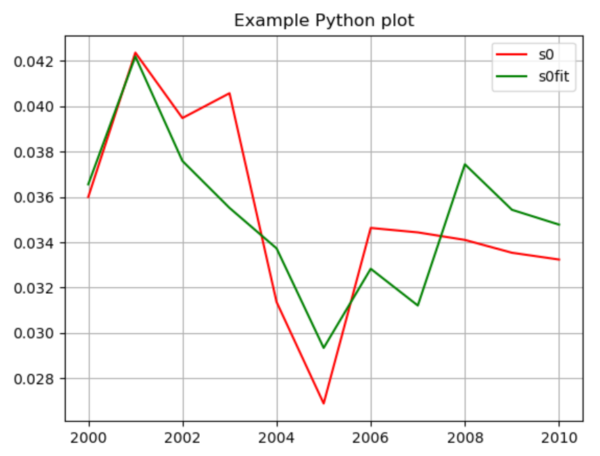
The program prints Python output on the screen, and plots actual and predicted values. Plotting is done using both Python's Matplotlib, and Gekko's own PLOT (the Python plot is shown below).

clip0040

The #beta vector looks like this:

#beta
   1
   1 0.0298
   2 0.1445
   3 0.6139
   4 0.1867
   5 -0.3509

Some of the output from Python shown in Gekko is the following (cf. the same example in the OLS section):

==============================================================================

coef std err t P>|t| [0.025 0.975]

------------------------------------------------------------------------------

const 0.0298 0.009 3.333 0.016 0.008 0.052

x1 0.1445 0.227 0.637 0.548 -0.411 0.700

x2 0.6139 0.236 2.596 0.041 0.035 1.193

x3 0.1867 0.203 0.922 0.392 -0.309 0.682

x4 -0.3509 0.203 -1.727 0.135 -0.848 0.146

==============================================================================

Omnibus: 1.122 Durbin-Watson: 1.865

Prob(Omnibus): 0.571 Jarque-Bera (JB): 0.895

Skew: 0.544 Prob(JB): 0.639

Kurtosis: 2.122 Cond. No. 253.

==============================================================================

Note that in this example, the <target= 'data1'> option and the corresponding gekkoimport data1 in the ols.py file are not really necessary, since the data could just be put at the top of the Python file anyway. The code that is injected into the Python file before it is executed looks like the following:

x = numpy.array([[0.0304674549413991,0.0206121780628441, ...], ...])
y = numpy.array([[0.0360024370055795],[0.0423704884205201], ... ])

And the file that Python produces for Gekko to consume looks like the following (this is actually what the gekkoexport() function in Python does):

Python2Gekko version 1.0

------------------------

name = beta

rows = 5

cols = 1

0.0298038917827622

0.1445172984105897

0.6138751350035226

0.18674011629660836

-0.35090825010498294

-------------------

...

This text-based way of interchanging data back and forth works fine, as long as the datasets are not too voluminous (otherwise see the following section). The interface is more stable than COM-based automation, and interchange of values, text, etc. could also be provided if needed.

Apache Arrow files

As an alternative to matrix-based communication with Python, Gekko also supports the so-called Apache Arrow format. This is a dataframe-like format that can be understood by R, Python, Julia, Matlab and many others. In the longer run, Gekko will provide dataframes, too, but for the moment it is possible to write/export all timeseries from a Gekko databank (or subset of a databank) to an arrow file for consumption in, say, R or Python. At the moment, only series can be exported as arrow files, metadata is not included, and IMPORT<arrow> does not work yet (will soon). The Arrow interface may change, so please do not yet use the interface in "serious" production code. There is a tremendous potential in the Arrow project regarding easy, fast and reliable transfer of data between software packages. (See the equivalent R example under R_RUN).

The following is a simple demo, highlighting some of the capabilities.

First, store the following test1.py file in your working folder:

# first time use, first install the Apache Arrow package:
# "pip install pyarrow" or "conda install -c conda-forge pyarrow"
import pandas as pd
df1 = pd.read_feather('test1.arrow')
print(df1)
df2 = df1.loc[df1['dims'] == 0][['name', 'freq', 'per1', 'value']]
print(df2)

Next, run the following Gekko statements:

reset; time 2021 2023;
x = 1, 2, 3;
series x1 = series(1); //1-dim array-series
x1[i] = 2, 3, 4;
x1[j] = 3, 4, 5;
series x2 = series(2); //2-dim array-series
x2[x, y] = 4, 5, 6;
x2[x, z] = 5, 6, 7;
export <arrow> test1.arrow;
python_run test1.py;

The data consists of a normal series x, a 1-dimensional array-series x1, and a 2-dimensional array-series x2. The following Python-output is shown in Gekko, after the test1.arrow file is read by Python:

name freq dims dim1 dim2 per1 value
0 x a 0 None None 2021 1.0
1 x a 0 None None 2022 2.0
2 x a 0 None None 2023 3.0
3 x1 a 1 i None 2021 2.0
4 x1 a 1 i None 2022 3.0
5 x1 a 1 i None 2023 4.0
6 x1 a 1 j None 2021 3.0
7 x1 a 1 j None 2022 4.0
8 x1 a 1 j None 2023 5.0
9 x2 a 2 x y 2021 4.0
10 x2 a 2 x y 2022 5.0
11 x2 a 2 x y 2023 6.0
12 x2 a 2 x z 2021 5.0
13 x2 a 2 x z 2022 6.0
14 x2 a 2 x z 2023 7.0

name freq per1 value
0 x a 2021 1.0
1 x a 2022 2.0
2 x a 2023 3.0

The first dataframe (df1) consists of all the data. The columns have the names name, freq, dims, dim1, dim2, per1, and value. These are either strings, integers or double precison numbers. In the dataframe None represents missing data. The name and freq represent the Gekko name (for instance x!a), and dims represents the number of dimensions. Columns dim1 and dim2 are the two potential dimensions, per1 is the year (for daily frequency there will be a per2 representing month, and per3 representing day), and value is the observation.

In the second dataframe (df2), dims == 0 is selected (that is, selecting only normal timeseries), and only columns name, freq, per1, value are shown. This resembles a more Gekko-like print of the x timeseries. EXPORT<arrow> supports all Gekko frequencies, but the particular dataframe layout may change.

Note

Note that with python_run<mute>, you will not see any potential Python errors on the screen. So please do not use <mute> when you are still debugging the Python program.

Note that at the moment, the gekkoexport() function only takes one argument/matrix at the time. The gekkoexport() function will work with simple names, else you must indicate the name as a string, for instance gekkoexport(results.params, 'beta').

You need to have Python installed on your computer. Gekko will try to auto-detect the location of Python from the Windows PATH, otherwise you may indicate the path via this option: option python exe folder = ... ; (Gekko will automatically add python.exe or \python.exe, unless the path ends with .exe, .bat or .cmd). To locate your python.exe file location, you may try this in Python: import sys; print(sys.executable) (this works for Python 3, for Python 2 you must omit the parentheses).

You can also use EXPORT<python> to export matrices to a file suitable for Python.

Related options

OPTION python exe folder = ... ; //you may use this, if the auto-detection of the location of Python fails

Related statements

R_RUN, OLS, MATRIX, EXPORT<python>, EXPORT<arrow>