|
<< Click to Display Table of Contents >> Goal-search etc. |
  
|
|
<< Click to Display Table of Contents >> Goal-search etc. |
|
In order to follow the examples, you must first download the model and databank (click demo.zip and copy the two files gekko.frm and gekko.gbk into your Gekko working folder).
(See the bottom of this page for the full code).
Start up Gekko in the working folder, and type:
restart; |
This clears up the workspace, and sets the global time period (for which we will later simulate the model). Next, issue these statements, in order to run the baseline simulation with 0% growth in government consumption.
model gekko; |
Gekko can do goals/means analysis, i.e. exogenizing some endogenous variables, and endogenizing some exogenous variables. In other words: force some endogenous variables to attain specific values, by means of some other (exogenous) variables. In this scenario, how would you augment y with 250 units for a 7-year period relative to the baseline scenario, by means of changing g? This experiment is done quite easily, via the EXO and ENDO statements:
exo y; |
These statements state that y should be redefined as an exogenous (goal) variable, whereas g is redefined as an endogenous variable (means). Note that when you simulate, the number of exogenized and endogenized variables should always be the same, otherwise Gekko will complain. Note also that a small target icon appears at the bottom right, to remind you that goals/means are set. After this, try to change y:
y <2017 2023> += 250; |
You get a warning that you are updating a left-hand side variable. Now simulate (we assume the global time period is still 2017-2040):
sim<fix>; |
To make the means/goals bind, you must use the <fix> option in the SIM statement. Plot the simulated variables (multiplier):
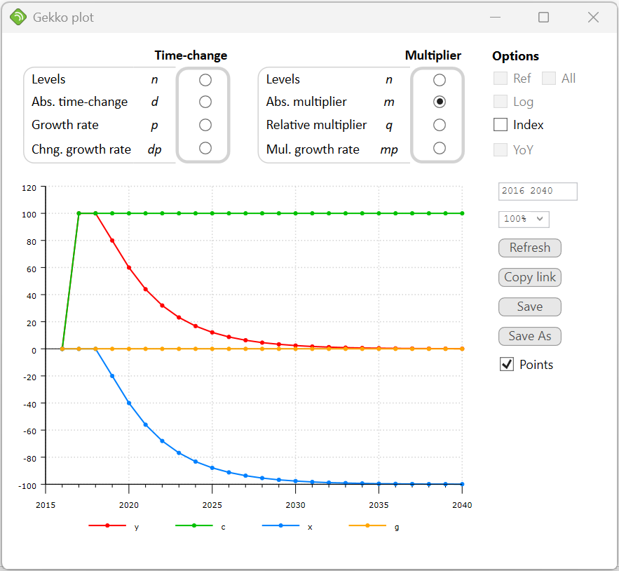
plot <2016 2040 m> y, c, x, g; |

It is seen that in order to keep the production level 250 units higher for 7 consecutive years, government spending has to keep growing continually up to 2023. In that period, net exports (x) get squeezed out, and the effect on x is negative from 2019 on (implying a likely trade deficit, depending upon the price of imports and exports). When the y-effect ends after 2023, g stays at a permanently higher level (350 units higher). The mirror-image of this is that net exports has diminished by the same amout (-350). You may compare this graph to the similar experiment in section 4.
To deactivate all goals/means, simply use SIM instead of SIM<fix>, or use the UNFIX statement to remove the goals/means completely.
If you want to fix a certain endogenous variable at some predefined value, by means of its add-factor, you may use ENDO/EXO for that, too. But in that case, there is an often more convenient method, namely using the so-called exogenization dummies. If the equation has a formula code implying exogenization dummy (the character D at the 5th position), this is possible.
The private consumption function c has code _GJ_D, implying that it has an additive add-factor (the J_ part of the code), and exogenization dummy (the last D in the code). So the "full" c-equation really is c = (0.6*y + 0.1*c[-1] + Jc) * (1-Dc) + Dc*Zc. The J_ part of the code "produces" the add-factor Jc, whereas the last D in the code "produces" the terms containing the variables Dc and Zc. The variable Dc is an exogenization dummy (normally 0), and the variable Zc can be used to set a value for c (if Dc = 1, the equation reduces to c = Zc).
Try starting from scratch with the scenario again (you may mark a block of statements and run them all when you hit [Enter]):
restart; |
Now try the following statements:
Dc = 1; |
As you can see, c is now fixed at a value 100 higher than in the baseline databank. In the long run this crowds out net exports x, so that GDP (y) is unchanged near 2040. The functionality can for instance be used in forecasts, if some observations of endogenous variables are known ahead of time (possibly tentatively, from other sources, indicators etc.).
At this point it should also be mentioned that it is possible to re-endogenize the variable c in a convenient fashion. If, after the above simulation, Dc is set to 0 again, and the model simulated, one would expect c to return to its previous values. This is not the case however: the value of c would stay at +100, even though the dummy has been set back. The explanation is that the add-factor Jc is calculated in a way so that the c-equation keeps it’s goal values. This trick of switching the dummy back and forth while simulating is quite advanced, and should only be used if the user fully understands the implications.
As you may have noted, in order to solve this goals/means problem, Gekko had to switch to another solving algorithm (Newton). This is done automatically, when EXO and ENDO statements are used. The Newton algorithm is more powerful that the Gauss algorithm (and allows changing the set of endogenous/exogenous variables). But for "normal" non-exogenized models, Newton is a bit slower, so for normal (non-goal) purposes, the Gauss algorithm is typically used.
If, however, you encounter solving problems with the Gauss algoritm, try switching to the Newton algorithm manually (option solve method = newton;). Also, the Newton algorithm is much more precise. This has to do with the fact that for each extra iteration, the Newton algorithm doubles the number of correct significant digits in the values of the endogenous variables. Gekko is designed for large-scale models, so you may indicate hundreds or thousands of simultaneous goals/means at the same time, if you like.
It should perhaps be noted that some kinds of equations can never be solved by means of a Gauss-Seidel algorithm, no matter how much damping etc. might be used. An example could be the one-equation model z = 1.1*z – 0.2*h. This model has the solution z = 2*h, but this solution can only be found with the Newton algorithm. If such equations are present in a model (possibly in hidden form), the solution space becomes a saddle point, and that requires a Newton solver. However, many macroeconomic models solve just fine with the (faster) Gauss solver.
The full code
restart; model gekko; exo y; y <2017 2023> += 250; sim<fix>; plot <2016 2040 m> y, c, x, g;
// -------------------------------
restart; Dc = 1; |