<< Click to Display Table of Contents >> Navigation:  Gekko User Guide > Modeling User Guide > Forward-looking

Gekko can handle forward-looking models, that is, models where one or more of the endogenous variables contain leads. There are different solvers regarding this, see under SIM, and also under option solve forward ... . We will first try to perform a multiplier analysis without leaded variables, similar to the shock shown in section 4:

 

 

If you copy-paste these statements to Gekko, you may either execute them individually one by one by pressing [Enter], or first mark them as a block and then press [Enter] to execute them at once. The "multiplier" (difference between the two simulations) looks like this:

 

 

This is the same effects as seen in section 4, were in this case, g is not augmented until the year 2025. In the model (gekko.frm), there is the following equation:

 

 

So if y is augmented by 1, c will augment by 0.6 in the same year. We will now create a new model with a different equation regarding consumption, c.

 

•In the file system, make a copy of gekko.frm and call it gekko2.frm

•In gekko2.frm, in the c equation, change 0.6*y into 0.6*y[+1].

 

So the equation now looks like this:

 

 

This means that current consumption, c, now reacts to the expected income next period, y[+1]. Next, run the following code:

 

 

 

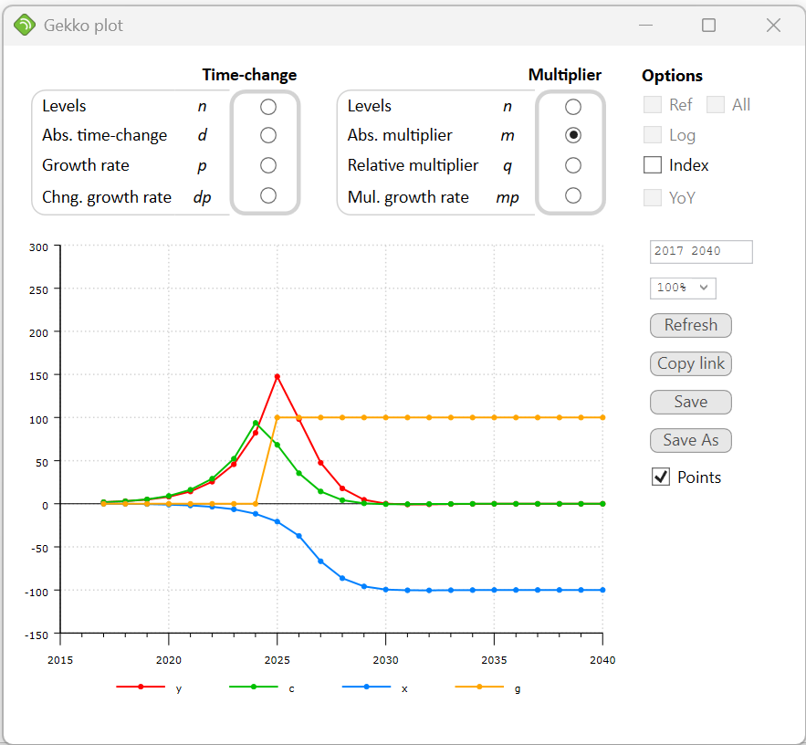
This is quite different from before, and it is seen that both c and y start to increase well before g increases in 2025. In the figure, it is seen that c now reacts to y in the next  period, for instance y decreases from 2025 to 2026, and hence c decreases the year before that, from 2024 to 2025.

 

In the above code, we have set y[2041] = 500, since this is the long-run equilibrium value (the only value for which the equation dif(x) = -0.2*(y[-2] - 500) is stationary). Hence, we are setting the terminal condition manually for this problem.